Introduction
This document provides a comprehensive reference for all the environmental variables available in the envar R package and the sources from which they can be retrieved. Each section describes a data source, lists the available variables with their synonyms, provides usage examples, and includes proper citations. Sources are grouped based on the category to which they belong (e.g., land cover, climate, etc.). For each source, the available variables are listed alongside synonyms that can be used inside the vars argument interchangeably (except for the chelsa and worldclim functions that do not allow the use of synonyms and the exact codes must be used).
Load package
When executing this command, another package (dplyr)
will be automatically loaded to ensure the full functionality of the
package. However, other packages are often required for plotting and
further analyses and we also load them here for later use.
Climate
CHELSA
This function downloads, processes, and extracts variables from the CHELSA (Climatologies at High Resolution for the Earth’s Land Surface Areas) dataset (Karger et al. 2017) and the CHELSA BIOCLIM+ dataset (Brun et al. 2022).
The following variables are available. Please note the distinction between “Monthly” time-series data and “Climatologies”. There is only one code-name for each variable and no working synonyms, differently from most other functions of the package, and in parentheses is the meaning. Climatologies are available for 30-year periods: 1981-2010, 2011-2040, 2041-2070, 2071-2100.
Available variables (67 total)
Monthly time-series (Available years: 1980 - 2018):
- 1 - pr (Precipitation amount; mass per unit area)
- 2 - tas (Mean daily air temperature at 2 meters)
- 3 - tasmax (Mean daily maximum air temperature at 2 meters)
- 4 - tasmin (Mean daily minimum air temperature at 2 meters)
- 5 - hurs (Near-surface relative humidity)
- 6 - clt (Total cloud cover at surface; considers entire atmospheric column)
- 7 - sfcWind (Near-surface wind speed at 10m above ground)
- 8 - vpd (Vapor pressure deficit)
- 9 - rsds (Surface downwelling shortwave flux in air)
- 10 - pet_penman (Potential evapotranspiration; Penman-Monteith equation)
- 11 - cmi (Climate Moisture Index)
- 12 - swb (Site water balance; cumulative available water)
Cloud Cover climatologies:
- 13 - clt_mean (Mean monthly total cloud cover over 1 year)
- 14 - clt_max (Maximum monthly total cloud cover)
- 15 - clt_min (Minimum monthly total cloud cover)
- 16 - clt_range (Annual range of monthly total cloud cover)
Climate Moisture Index climatologies:
- 17 - cmi_mean (Mean monthly climate moisture index)
- 18 - cmi_max (Maximum monthly climate moisture index; highest surplus)
- 19 - cmi_min (Minimum monthly climate moisture index; highest deficit)
- 20 - cmi_range (Annual range of monthly climate moisture index)
Relative humidity climatologies:
- 21 - hurs_mean (Mean monthly near-surface relative humidity)
- 22 - hurs_max (Maximum monthly near-surface relative humidity)
- 23 - hurs_min (Minimum monthly near-surface relative humidity)
- 24 - hurs_range (Annual range of monthly near-surface relative humidity)
Potential evapotranspiration climatologies:
- 25 - pet_penman_mean (Mean monthly PET)
- 26 - pet_penman_max (Maximum monthly PET)
- 27 - pet_penman_min (Minimum monthly PET)
- 28 - pet_penman_range (Annual range of monthly PET)
Solar radiation climatologies:
- 29 - rsds_mean (Mean monthly surface downwelling shortwave flux)
- 30 - rsds_max (Maximum monthly surface downwelling shortwave flux)
- 31 - rsds_min (Minimum monthly surface downwelling shortwave flux)
- 32 - rsds_range (Annual range of monthly surface downwelling shortwave flux)
Wind speed climatologies:
- 33 - sfcWind_mean (Mean monthly near-surface wind speed)
- 34 - sfcWind_max (Maximum monthly near-surface wind speed)
- 35 - sfcWind_min (Minimum monthly near-surface wind speed)
- 36 - sfcWind_range (Annual range of monthly near-surface wind speed)
Vapor pressure deficit climatologies:
- 37 - vpd_mean (Mean monthly vapor pressure deficit)
- 38 - vpd_max (Maximum monthly vapor pressure deficit)
- 39 - vpd_min (Minimum monthly vapor pressure deficit)
- 40 - vpd_range (Annual range of monthly vapor pressure deficit)
Growing season characteristics (TREELIM model):
- 41 - gsl (Growing season length; days) *Note: Corrected from ‘gls’
- 42 - gsp (Accumulated precipitation during growing season)
- 43 - gst (Mean temperature of the growing season)
- 44 - fgd (First day of the growing season; Julian day)
- 45 - lgd (Last day of the growing season; Julian day)
Growing Degree Days (GDD):
46 - gdd0 (Heat sum of all days > 0°C accumulated over 1 year)
47 - gdd5 (Heat sum of all days > 5°C accumulated over 1 year)
48 - gdd10 (Heat sum of all days > 10°C accumulated over 1 year)
49 - ngd0 (Number of days with tas > 0°C)
50 - ngd5 (Number of days with tas > 5°C)
51 - ngd10 (Number of days with tas > 10°C)
52 - gdgfgd0 (First growing degree day > 0°C; Julian day)
53 - gdgfgd5 (First growing degree day > 5°C; Julian day)
54 - gdgfgd10 (First growing degree day > 10°C; Julian day)
55 - gddlgd0 (Last growing degree day > 0°C; Julian day)
56 - gddlgd5 (Last growing degree day > 5°C; Julian day)
57 - gddlgd10 (Last growing degree day > 10°C; Julian day)
Snow and frost climatologies:
- 58 - scd (Snow cover days; count)
- 59 - swe (Snow water equivalent; accumulated amount of liquid water if snow melted)
- 60 - fcf (Frost change frequency; events where tmin/tmax cross 0°C)
Biological productivity:
- 61 - npp (Net primary productivity; g C m^-2 yr^-1)
Climate classifications (Köppen-Geiger & others):
- 62 - kg0 (Köppen-Geiger climate category)
- 63 - kg1 (Köppen-Geiger without As/Aw differentiation)
- 64 - kg2 (Köppen-Geiger after Peel et al. 2007)
- 65 - kg3 (Wissmann 1939 classification)
- 66 - kg4 (Thornthwaite 1931 classification)
- 67 - kg5 (Troll-Pfaffen classification)
It is necessary to specify also the years as a distinct argument. If specified as a range (e.g. “1981-2010”) the average of those years is downloaded, otherwise if a single year is specified, the variables will refer to that year. With the argument “months” (numeric vector from 1 to 12) it is also possible to download data only for one or multiple specified months. If this is parameter is not specified, 12 months will be downloaded as 12 distinct layers. When downloading future variables across all possible CHELSA downloads, it is also necessary to specify the general circulation model(s) within the “gcm” argument, the representation concentration pathway(s) with “rcp”, and the shared socioeconomic pathway with the “ssp” argument. If the year(s) and gcm(s) and ssp(s) are not specified properly or not specified at all, the download will not work.
plot(processed[[1]])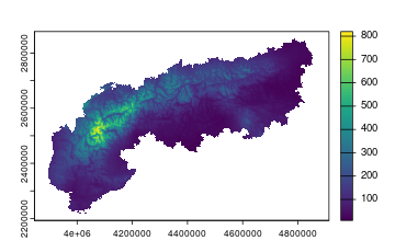
plot of chunk unnamed-chunk-5
WorldClim
This function downloads, processes, and extracts variables from the WorldClim climate dataset (Fick & Hijmans 2017). Each variable corresponds to a global raster representing climate variables at approximately 1-km resolution. It supports both Historical (v2.1, 1970-2000) and Future (CMIP6) data.
Available variables (8 total)
Temperature:
- 1 - tmin - min temp
- 2 - tmax - max temp
- 3 - tavg - average temp
Precipitation:
- 4 - prec - precipitation, pr
Physical:
- 5 - srad - solar radiation
- 6 - wind - wind speed
- 7 - vapr - water vapor
- 8 - elev - elevation
Bioclimatic:
- bio - All 19 bioclimatic variables
- bio1 - bio19 - Specific bioclimatic variables
Historical:
- 1970-2000 (or “historical”)
Future:
- 2021-2040
- 2041-2060
- 2061-2080
- 2081-2100
Climate zones
This function downloads, processes, and extracts variables from the High-resolution (1 km) Köppen-Geiger maps dataset (Beck et al. 2023). Each variable corresponds to a global GeoTIFF representing climate classification zones based on historical data or future CMIP6 projections.
Available variables (1 total)
- 1 - zones - koppengeiger, climate, climatezones, koppen, koppen geiger
Time periods (“years” argument):
Historical:
- 1901-1930
- 1931-1960
- 1961-1990
- 1991-2020 (default)
Future:
- 2041-2070
- 2071-2099
SSP Scenarios (“ssp” argument, required for future periods):
- 119 (SSP1-1.9)
- 126 (SSP1-2.6)
- 245 (SSP2-4.5)
- 370 (SSP3-7.0)
- 434 (SSP4-3.4)
- 460 (SSP4-6.0)
- 585 (SSP5-8.5)
processed <- par_set(shape = Alps, crs = 3035) %>%
  climatezones()
plot(processed[[1]])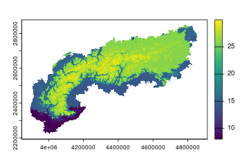
plot of chunk unnamed-chunk-8
Cloud cover
This function downloads, processes, and extracts variables from the EarthEnv Global Cloud Cover dataset (Wilson & Jetz 2016). Each variable corresponds to a global Cloud-Optimized GeoTIFF (COG) representing cloud cover dynamics.
Available variables (21 total)
Metrics:
- 1 - MODCF_CloudForestPrediction - cloud forest prediction, cloud forest, cfp
- 2 - MODCF_interannualSD - inter-annual variability, interannual sd, interannual variability
- 3 - MODCF_intraannualSD - intra-annual variability, intraannual sd, intraannual variability
- 4 - MODCF_meanannual - mean annual, annual mean, annual
- 5 - MODCF_spatialSD_1deg - spatial variability, spatial sd, spatial sd 1deg
Seasonality:
- 6 - MODCF_seasonality_concentration - seasonality concentration, concentration
- 7 - MODCF_seasonality_rgb - seasonality rgb, rgb
- 8 - MODCF_seasonality_theta - seasonality theta, theta
- 9 - MODCF_seasonality_visct - seasonality single band, seasonality visct, seasonality color
Monthly means:
- 10 - MODCF_monthlymean_01 - january mean, january, jan
- 11 - MODCF_monthlymean_02 - february mean, february, feb
- 12 - MODCF_monthlymean_03 - march mean, march, mar
- 13 - MODCF_monthlymean_04 - april mean, april, apr
- 14 - MODCF_monthlymean_05 - may mean, may
- 15 - MODCF_monthlymean_06 - june mean, june, jun
- 16 - MODCF_monthlymean_07 - july mean, july, jul
- 17 - MODCF_monthlymean_08 - august mean, august, aug
- 18 - MODCF_monthlymean_09 - september mean, september, sep
- 19 - MODCF_monthlymean_10 - october mean, october, oct
- 20 - MODCF_monthlymean_11 - november mean, november, nov
- 21 - MODCF_monthlymean_12 - december mean, december, dec
processed <- par_set(shape = Alps, crs = 3035) %>%
  cloudcover(vars = c("mean annual"))
plot(processed[[1]])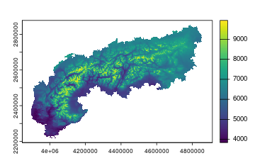
plot of chunk unnamed-chunk-10
Aridity
This function downloads, processes, and extracts variables from the Global Aridity Index and ET0 Database v3 (Zomer et al. 2022). Each variable corresponds to a global raster representing aridity index or potential evapotranspiration values.
Available variables (27 total)
Annual variables:
- 1 - ai_v3_yr.tif - aridity index annual, ai annual, aridity annual, ai year
- 2 - et0_v3_yr.tif - et0 annual, potential evapotranspiration annual, evapotranspiration annual, et0 year
- 3 - et0_v3_yr_sd.tif - et0 standard deviation, et0 sd, et0 variability, et0 annual sd
Monthly Aridity Index (ai_v3_01.tif to ai_v3_12.tif):
- 4 - ai_v3_01.tif - aridity index january, ai january, ai jan, ai 1
- 5 - ai_v3_02.tif - aridity index february, ai february, ai feb, ai 2
- 6-15 - … (continues for all 12 months)
Monthly ET0 (et0_v3_01.tif to et0_v3_12.tif):
- 16 - et0_v3_01.tif - et0 january, potential evapotranspiration january, et0 jan, et0 1
- 17 - et0_v3_02.tif - et0 february, potential evapotranspiration february, et0 feb, et0 2
- 18-27 - … (continues for all 12 months)
processed <- par_set(shape = Alps, crs = 3035) %>%
  aridity(vars = c("aridity index annual", "et0 january"))
plot(processed[[1]])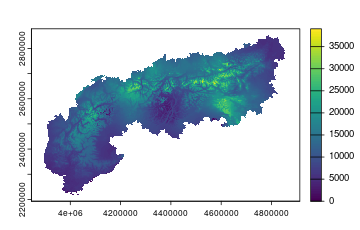
plot of chunk unnamed-chunk-12
Land cover
EarthEnv land cover
This function downloads, processes, and extracts variables from the EarthEnv Consensus Land Cover dataset (Tuanmu & Jetz 2014). Each variable corresponds to a global raster representing a specific land cover class at 1 km resolution.
Available variables (12 total)
- 1 - consensus_full_class_1 - evergreen deciduous needleleaf trees, needleleaf trees, needleleaf, conifer
- 2 - consensus_full_class_2 - evergreen broadleaf trees, evergreen broadleaf, broadleaf evergreen
- 3 - consensus_full_class_3 - deciduous broadleaf trees, deciduous broadleaf, broadleaf deciduous
- 4 - consensus_full_class_4 - mixed other trees, mixed trees, other trees, mixed forest
- 5 - consensus_full_class_5 - shrubs, shrubland, shrub
- 6 - consensus_full_class_6 - herbaceous vegetation, herbaceous, grassland, grass, herbs
- 7 - consensus_full_class_7 - cultivated and managed vegetation, cultivated, managed vegetation, agriculture, crops, cropland
- 8 - consensus_full_class_8 - regularly flooded vegetation, flooded vegetation, flooded, wetland
- 9 - consensus_full_class_9 - urban built up, urban, built up, built-up, artificial surface
- 10 - consensus_full_class_10 - snow ice, snow, ice, glacier, permafrost
- 11 - consensus_full_class_11 - barren, barren land, bare ground, bare
- 12 - consensus_full_class_12 - open water, water, water bodies
processed <- par_set(shape = Alps, crs = 3035) %>%
  earthenvlandcover(vars = c("snow ice"))
plot(processed[[1]])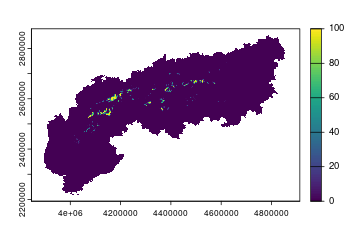
plot of chunk unnamed-chunk-14
Macroecological Land Cover
This function downloads, processes, and extracts variables from the Global 1 km Land Cover dataset (Lo Parrino et al. 2025). Each variable corresponds to a global raster representing a specific land cover class or diversity index derived from very high-resolution imagery.
Available variables (15 total)
- 1 - wetland - wetlands, swamp, marsh, bog, fen
- 2 - bare - bare ground, bare soil, desert, unvegetated
- 3 - built - built area, built up, urban, artificial, impervious
- 4 - cropland - agriculture, agricultural, crop, crops, farming
- 5 - grass - grassland, grass land, meadow, pasture, prairie
- 6 - ice - snow, snow and ice, glacier, ice, permafrost
- 7 - land_perc - percentage of land, land percentage, land cover fraction, land fraction
- 8 - mangrove - mangroves
- 9 - moss - mosses, lichen, lichens, moss and lichen
- 10 - shrub - shrubland, scrub, bush, thicket
- 11 - tree - trees, forest, woodland, canopy, canopy cover
- 12 - water - surface water, lake, river, freshwater
- 13 - simpson - simpson index, diversity simpson, simpson diversity
- 14 - shannon - shannon index, entropy, shannon entropy, shannon diversity
- 15 - evenness - evenness index, pielou, pielou evenness, species evenness
plot(processed[[1]])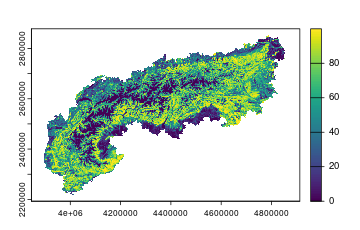
plot of chunk unnamed-chunk-16
Hybrid land cover
This function downloads, processes, and extracts land cover variables from the Hybrid Global Annual 1-km IGBP Land Cover Maps dataset (Luo et al. 2024). The data covers the period from 2000 to 2020.
Available variables (1 total)
- 1 - landcover - cover, land, lc, igbp, hybrid
Note: If the vars argument is left empty, the function
will default to downloading the land cover map. You must specify the
year argument (integer between 2000 and 2020).
processed <- par_set(shape = Alps, crs = 3035) %>%
  hybridlandcover(vars = "landcover", year = 2015)
plot(processed[[1]])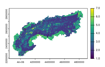
plot of chunk unnamed-chunk-18
GeoSOS land cover
This function downloads, processes, and extracts variables from the Global Land-Use and Land-Cover Change Product (2010-2100) (Li et al. 2017). The dataset provides global 1 km resolution rasters based on different IPCC scenarios.
Land cover classification legend:
- 1: Water
- 2: Forest
- 3: Grassland
- 4: Farmland
- 5: Urban
- 6: Barren
Available variables (1 total)
- 1 - landcover - lc, cover, land cover, land use, lulc, classes
Available scenarios (for years > 2010; 2010 is from MODIS baseline landcover):
- A1B
- A2
- B1
- B2
Available years:
- 2010
- 2050
- 2100
processed <- par_set(shape = Alps, crs = 3035) %>%
  geososlandcover(vars = "landcover", scenario = "A1B", year = 2050)
plot(processed[[1]])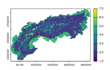
plot of chunk unnamed-chunk-20
PFT land cover
This function downloads, processes, and extracts land cover variables from the Global 7-land-types LULC projection dataset based on Plant Functional Types (PFT) with a 1-km resolution under socio-climatic scenarios (Chen et al. 2022b).
Available variables (1 total)
- 1 - landcover - cover, land, lulc, pft, projection
Note: If the vars argument is left empty, the function
will default to downloading the land cover map.
Required arguments:
year: Integer. Available years: 2020 to 2100 in 5-year
intervals (2020, 2025, 2030, …, 2100).
ssp: Integer or character. The SSP-RCP scenario code.
Available values:
- 119 (SSP1-RCP1.9)
- 126 (SSP1-RCP2.6)
- 245 (SSP2-RCP4.5)
- 370 (SSP3-RCP7.0)
- 434 (SSP4-RCP3.4)
- 460 (SSP4-RCP6.0)
- 534 (SSP5-RCP3.4)
- 585 (SSP5-RCP8.5)
processed <- par_set(shape = Alps, crs = 3035) %>%
  pftlandcover(vars = "landcover", year = 2050, ssp = 585)
plot(processed[[1]])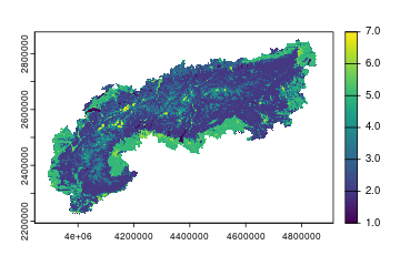
plot of chunk unnamed-chunk-22
GCAM land cover
This function downloads, processes, and extracts simulated global land use and land cover (LULC) data for the period 2020-2100 (Gao et al. 2025).
The data represents 1 km resolution LULC maps with the following integer codes:
- 1: Cropland
- 2: Forest
- 3: Grassland
- 4: Urban
- 5: Barren
- 6: Water
Available variables (1 total)
- 1 - landcover - The specific map is determined by
the
yearandssparguments
Available years:
- 2020
- 2030
- 2050
- 2070
- 2100
Available SSPs (Shared Socioeconomic Pathways):
- 126 (SSP1-2.6)
- 245 (SSP2-4.5)
- 370 (SSP3-7.0)
- 434 (SSP4-3.4)
- 585 (SSP5-8.5)
Note: The original data is in World Mercator projection and will be
automatically reprojected to the CRS defined in par_set()
(default: EPSG 4326).
processed <- par_set(shape = Alps, crs = 3035) %>%
  gcamlandcover(ssp = 585, year = 2050)
plot(processed[[1]])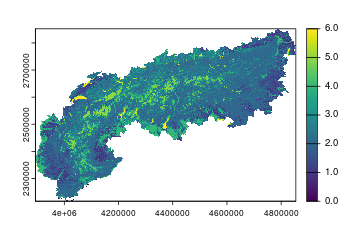
plot of chunk unnamed-chunk-24
Landscape heterogeneity
This function downloads, processes, and extracts variables from the EarthEnv habitat heterogeneity dataset (1-km resolution) (Tuanmu & Jetz 2015). Each variable corresponds to a global Cloud-Optimized GeoTIFF (COG) representing different metrics of habitat heterogeneity derived from remote sensing data.
Available variables (14 total)
First-order statistics:
- 1 - cv - coefficient of variation, coeff of variation
- 2 - evenness - even
- 3 - range - range
- 4 - shannon - shannon index, shannon entropy
- 5 - simpson - simpson index, simpson diversity
- 6 - std - standard deviation, std dev
Second-order statistics (Texture metrics):
- 7 - Contrast - contrast
- 8 - Correlation - correlation, corr
- 9 - Dissimilarity - dissimilarity
- 10 - Entropy - entropy, texture entropy
- 11 - Homogeneity - homogeneity
- 12 - Maximum - maximum, max
- 13 - Uniformity - uniformity, uniform
- 14 - Variance - variance, var
processed <- par_set(shape = Alps, crs = 3035) %>%
  heterogeneity(vars = c("shannon", "cv"))
plot(processed[[1]])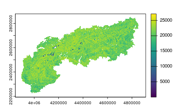
plot of chunk unnamed-chunk-26
Habitats
This function downloads, processes, and extracts variables from the IUCN Global Habitat Classification Fractions dataset (Jung et al. 2020). The data is available at Level 1 (broad) and Level 2 (detailed) classifications.
Available variables (Level 1 - 12 total)
- 1 - 100_Forest - forest, 100
- 2 - 200_Savanna - savanna, 200
- 3 - 300_Shrubland - shrubland, 300
- 4 - 400_Grassland - grassland, 400
- 5 - 500_Wetlands inland - wetlands inland, wetlands, inland wetlands, 500
- 6 - 600_Rocky Areas - rocky areas, rocky, 600
- 7 - 800_Desert - desert, 800
- 8 - 900_Marine - Neritic - marine neritic, neritic, 900
- 9 - 1000_Marine - Oceanic - marine oceanic, oceanic, 1000
- 10 - 1100_Marine - Deep Ocean Floor - marine deep ocean floor, deep ocean floor, 1100
- 11 - 1200_Marine - Intertidal - marine intertidal, intertidal, 1200
- 12 - 1400_Artificial - Terrestrial - artificial terrestrial, artificial, terrestrial artificial, 1400
Available variables (selection from Level 2 - check original paper for a more careful description and complete list)
Forests:
- 1 - 101_Forest - Boreal - forest boreal, boreal forest, 101
- 2 - 104_Forest - Temperate - forest temperate, temperate forest, 104
- 3 - 105_Forest - Subtropical-tropical dry - forest subtropical tropical dry, dry forest, tropical dry forest, 105
- 4 - 106_Forest - Subtropical-tropical moist lowland - forest subtropical tropical moist lowland, moist lowland forest, tropical moist forest, 106
- 5 - 107_Forest - Subtropical-tropical mangrove vegetation - forest mangrove, mangrove, mangroves, 107
- 6 - 108_Forest - Subtropical-tropical swamp - forest swamp, swamp forest, tropical swamp, 108
- 7 - 109_Forest - Subtropical-tropical moist montane - forest moist montane, montane forest, cloud forest, 109
Savannas:
- 8 - 201_Savanna - Dry - savanna dry, dry savanna, 201
- 9 - 202_Savanna - Moist - savanna moist, moist savanna, 202
Shrublands:
- 10 - 303_Shrubland - Boreal - shrubland boreal, boreal shrubland, 303
- 11 - 304_Shrubland - Temperate - shrubland temperate, temperate shrubland, 304
- 12 - 305_Shrubland - Subtropical-tropical dry - shrubland dry, tropical dry shrubland, 305
- 13 - 306_Shrubland - Subtropical-tropical moist - shrubland moist, tropical moist shrubland, 306
- 14 - 308_Shrubland - Mediterranean-type - shrubland mediterranean, mediterranean shrubland, 308
Grasslands:
- 15 - 401_Grassland - Tundra - grassland tundra, tundra, 401
- 16 - 404_Grassland - Temperate - grassland temperate, temperate grassland, 404
- 17 - 405_Grassland - Subtropical-tropical dry - grassland dry, tropical dry grassland, 405
- 18 - 1402_Pastureland - pastureland, pasture
Wetlands:
- 19 - 501_Wetlands inland - Permanent rivers-streams-creeks - rivers, streams, creeks, 501
- 20 - 504_Wetlands inland - Bogs, marshes, swamps, fens, peatlands - bogs, marshes, swamps, fens, peatlands, 504
- 21 - 505_Wetlands inland - Permanent freshwater lakes - freshwater lakes, lakes, 505
Deserts:
- 22 - 801_Desert - Hot - desert hot, hot desert, 801
- 23 - 802_Desert - Temperate - desert temperate, temperate desert, 802
- 24 - 803_Desert - Cold - desert cold, cold desert, 803
Artificial:
- 25 - 1401_Arable Land - arable land, arable, 1401
- 26 - 1403_Plantations - plantations, plantation, 1403
- 27 - 1405_Urban Areas - urban areas, urban, 1405
processed <- par_set(shape = Alps, crs = 3035) %>%
  habitat(vars = c("Forest", "Artificial"), level = 1)
plot(processed[[1]])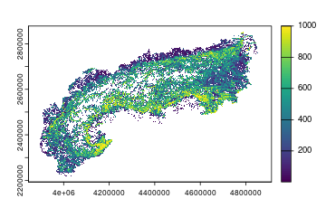
plot of chunk unnamed-chunk-28
Soil characteristics
Harmonized World Soil Database
This function downloads, processes, and extracts variables from the Harmonized World Soil Database v2.0 (HWSD v2.0) (authors 2023). The variable corresponds to a global raster file at 1 km resolution representing soil types.
Available variables (1 total)
- 1 - hwsd - soil, type, soiltype, soil type
plot(processed[[1]])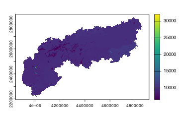
plot of chunk unnamed-chunk-30
Soil climate
This function downloads, processes, and extracts soil bioclimatic variables and monthly soil temperatures from the Global Soil Temperature dataset (Lembrechts et al. 2022).
Available variables (23 total)
Bioclimatic variables:
- 1 - SBIO1 - annual mean temperature, annual mean, amt
- 2 - SBIO2 - mean diurnal range, mean diurnal, mdr
- 3 - SBIO3 - isothermality, iso
- 4 - SBIO4 - temperature seasonality, seasonality, temp seasonality
- 5 - SBIO5 - max temperature warmest month, max temp, warmest month
- 6 - SBIO6 - min temperature coldest month, min temp, coldest month
- 7 - SBIO7 - temperature annual range, annual range, tar
- 8 - SBIO8 - mean temperature wettest quarter, wettest quarter
- 9 - SBIO9 - mean temperature driest quarter, driest quarter
- 10 - SBIO10 - mean temperature warmest quarter, warmest quarter
- 11 - SBIO11 - mean temperature coldest quarter, coldest quarter
Monthly mean soil temperatures:
- 12 - soilT01 - january mean, january, jan
- 13 - soilT02 - february mean, february, feb
- 14 - soilT03 - march mean, march, mar
- 15 - soilT04 - april mean, april, apr
- 16 - soilT05 - may mean, may
- 17 - soilT06 - june mean, june, jun
- 18 - soilT07 - july mean, july, jul
- 19 - soilT08 - august mean, august, aug
- 20 - soilT09 - september mean, september, sep
- 21 - soilT10 - october mean, october, oct
- 22 - soilT11 - november mean, november, nov
- 23 - soilT12 - december mean, december, dec
The depth argument defines the soil depth range in cm.
Options are “0-5” (default) or “5-15”.
processed <- par_set(shape = Alps, crs = 3035) %>%
  soilclimate(vars = c("SBIO1", "SBIO10"), depth = "5-15")
plot(processed[[1]])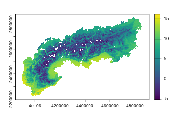
plot of chunk unnamed-chunk-32
Topography
This function downloads, processes, and extracts variables from the EarthEnv Topography dataset (Amatulli et al. 2018). This dataset provides global, cross-scale topographic variables suitable for biodiversity and ecosystem modeling.
Available variables (11 total)
- 1 - elevation - dem, height, alt, altitude
- 2 - slope - slope
- 3 - aspect - aspect
- 4 - roughness - rough
- 5 - tri - terrain ruggedness index, ruggedness
- 6 - tpi - topographic position index, position
- 7 - vrm - vector ruggedness measure
- 8 - pcurv - profile curvature, profile curve
- 9 - tcurv - tangential curvature, tangential curve
- 10 - eastness - east
- 11 - northness - north
Additional parameters:
- algorithm - Aggregation method/algorithm to use. Options: “md” (median, default), “mn” (mean), “min”, “max”, “sd”.
- topo_source - Data source. Options: “GMTED” (default) or “SRTM”.
processed <- par_set(shape = Alps, crs = 3035) %>%
  topography(vars = c("elevation", "slope"))
plot(processed[[1]])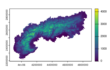
plot of chunk unnamed-chunk-34
Freshwater environments
This function downloads, processes, and extracts variables from the near-global freshwater-specific environmental variables dataset (Domisch et al. 2015). These variables are available at a 1 km resolution and capture upstream catchment characteristics, including topography, land cover, soil, and climate.
Available variables
The freshwater() function provides access to 324
near-global 1-km resolution layers. You can filter specific layers from
within these collections using the month argument (for
climatic variables) and algorithm argument (for
topographic, soil, and aggregation methods).
Temperature (monthly)
Use the month argument (1–12) to select specific months.
- 1 - monthly_tmin_average.nc – monthly minimum temperature average, min temp average, tmin avg, tmin
- 2 - monthly_tmax_average.nc – monthly maximum temperature average, max temp average, tmax avg, tmax
- 3 - monthly_tmin_weighted_average.nc – monthly minimum temperature weighted, min temp weighted, tmin weighted
- 4 - monthly_tmax_weighted_average.nc – monthly maximum temperature weighted, max temp weighted, tmax weighted
Precipitation
- 5 - monthly_prec_sum.nc – monthly upstream precipitation sum, precipitation sum, precip sum, prec
- 6 - monthly_prec_weighted_sum.nc – monthly upstream precipitation weighted, precipitation weighted, precip weighted
Hydroclimatic
- 7 - hydroclim_average+sum.nc – hydroclimatic variables average, hydroclim average, hydroclim
- 8 - hydroclim_weighted_average+sum.nc – hydroclimatic variables weighted, hydroclim weighted
Topography
- 9 - elevation.nc – upstream elevation, elevation, dem
- 10 - slope.nc – upstream slope, slope
- 11 - flow_acc.nc – stream length, flow accumulation, flow
Land cover
- 12 - landcover_minimum.nc – upstream landcover minimum, landcover min
- 13 - landcover_maximum.nc – upstream landcover maximum, landcover max
- 14 - landcover_range.nc – upstream landcover range, landcover range
- 15 - landcover_average.nc – upstream landcover average, landcover avg, landcover
- 16 - landcover_weighted_average.nc – upstream landcover weighted, landcover weighted
Geology & soil
- 17 - geology_weighted_sum.nc – upstream geology, geology weighted, geology
- 18 - soil_minimum.nc – upstream soil minimum, soil min
- 19 - soil_maximum.nc – upstream soil maximum, soil max
- 20 - soil_range.nc – upstream soil range, soil range
- 21 - soil_average.nc – upstream soil average, soil avg, soil
- 22 - soil_weighted_average.nc – upstream soil weighted, soil weighted
Quality control
- 23 - quality_control.nc – quality control, qc
Using the month argument
The month argument is used only for monthly variables (tmin, tmax, prec). Supplying one or several months filters the dataset to those corresponding monthly bands.
Using the algorithm argument
The algorithm argument filters specific statistical bands for topography, flow accumulation, soils, and land cover.
For elevation and slope layers, algorithms map to band order: * min – Band 1 * max – Band 2 * range – Band 3 * avg / mn – Band 4
Flow accumulation: * length – Band 1 (stream length) * acc – Band 2 (catchment accumulation)
For land cover and soil variables, the algorithm matches text patterns in filenames (e.g., “maximum”, “weighted”, “average”). When multiple variables are requested, the algorithm applies to the entire request, so multiple calls may be required if different algorithms are needed.
processed <- par_set(shape = Alps, crs = 3035) %>%
freshwater(vars = c("elevation", "slope", "tmin"), algorithm = "mn", month=12)
plot(processed[[3]])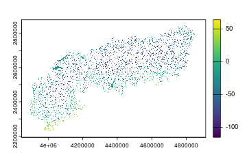
plot of chunk unnamed-chunk-36
Marine environments
This function downloads, processes, and extracts variables from the Bio-ORACLE v3.0 dataset (Assis et al. 2024).
Available variables (24 total)
- 1 - thetao - Ocean temperature [ºC] (temperature, temp, sea temperature)
- 2 - so - Salinity [-] (sal, salt, saltiness)
- 3 - sws - Sea water velocity [m.s-1] (velocity, current speed, speed)
- 4 - swd - Sea water direction [degree] (direction, current direction)
- 5 - no3 - Nitrate [mmol.m-3] (nitrate)
- 6 - po4 - Phosphate [mmol.m-3] (phosphate)
- 7 - si - Silicate [mmol.m-3] (silicate, silicon)
- 8 - o2 - Dissolved molecular oxygen [mmol.m-3] (oxygen, dissolved oxygen)
- 9 - dfe - Iron [mmol.m-3] (iron, fe)
- 10 - phyc - Primary productivity [mmol.m-3] (productivity, pp, primary production)
- 11 - ph - pH [-] (acidity)
- 12 - chl - Chlorophyll [mg.m-3] (chlorophyll, chla)
- 13 - sithick - Sea ice thickness [m] (ice thickness)
- 14 - siconc - Sea ice cover [Fraction] (ice cover, sea ice)
- 15 - clt - Cloud cover [%] (cloud, clouds)
- 16 - mlotst - Mixed layer depth [m] (mld, mixed layer)
- 17 - tas - Air temperature [ºC] (air temperature, air temp)
- 18 - par - Photosynthetically Available Radiation [E.m-2.day-1] (light, radiation)
- 19 - kdpar - Diffuse attenuation [m-1] (attenuation, turbidity)
- 20 - bathymetry - Bathymetry [m] (depth, elevation, altitude)
- 21 - slope - Topographic slope [-] (topographic slope)
- 22 - aspect - Topographic aspect [-] (topographic aspect)
- 23 - tpi - Topographic position index [-] (topographic position index)
- 24 - tri - Terrain ruggedness index [-] (terrain ruggedness index, ruggedness)
Additional parameters:
- realm - One of “surface” (default), “benthic_minimum”, “benthic_average”, or “benthic_maximum”
- years - Decade range (e.g., “2000-2010” up to “2090-2100”)
- ssp - Shared Socioeconomic Pathway for future projections (119, 126, 245, 370, 460, 585)
- algorithm - Statistic to apply (max, mean, min, ltmax, ltmin, range). Default “mean”
processed <- par_set(marine_ecoregion = "East African Coral Coast", res = 6) %>%
  biooracle(vars = "o2", realm = "surface", years = "2000-2010")
plot(processed[[1]])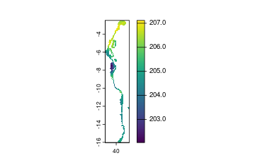
plot of chunk unnamed-chunk-38
Human impact
SPECTRE
This function downloads, processes, and extracts variables from the SPECTRE – Spatially Explicit ECosysTem ThREats dataset (Branco et al. 2024). Each variable corresponds to a global Cloud-Optimized GeoTIFF (COG) representing a different anthropogenic or climatic threat. When using this source, cite (Branco et al. 2024) and also the original source for each variable (check references in (Branco et al. 2024)).
Available variables (21 total)
Land use and human pressure:
- 1 - 1_1_MINING_AREA_cog - mining area, mining_area, mining
- 2 - 1_2_HAZARD_POTENTIAL_cog - hazard potential, hazard
- 3 - 1_3_HUMAN_DENSITY_cog - human density, population, pop
- 4 - 1_4_BUILT_AREA_cog - built area, built
- 5 - 1_5_ROAD_DENSITY_cog - road density, roads, road
- 6 - 1_6_FOOTPRINT_PERC_cog - human footprint, footprint
- 7 - 1_7_IMPACT_AREA_cog - impacted area, impact area
- 8 - 1_8_MODIF_AREA_cog - modified area, modif area
- 9 - 1_9_HUMAN_BIOMES_cog - human biomes, biomes
- 10 - 1_10_FIRE_OCCUR_cog - fires, fire
- 11 - 1_11_CROP_PERC_UNI_cog - crops uni, crop uni, crop
- 12 - 1_12_CROP_PERC_IIASA_cog - crops iiasa, iiasa crops
- 13 - 1_13_LIVESTOCK_MASS_cog - livestock, livestock mass
Forest loss:
- 14 - 2_1_FOREST_LOSS_PERC_cog - forest loss
- 15 - 2_2_FOREST_TREND_cog - forest trend
Light pollution:
- 16 - 3_1_LIGHT_MCDM2_cog - light at night, night light, light
Climate change:
- 17 - 5_1_TEMP_TRENDS_cog - temperature trends, temp trends
- 18 - 5_2_TEMP_SIGNIF_cog - temperature significance, temp signif
- 19 - 5_3_CLIM_EXTREME_cog - climate extremes
- 20 - 5_4_CLIM_VELOCITY_cog - climate velocity, velocity
- 21 - 5_5_ARIDITY_TREND_cog - aridity trend, aridity
processed <- par_set(shape = Alps, crs = 3035) %>%
  spectre(vars = c("forest loss", "light at night"))
plot(processed[[1]])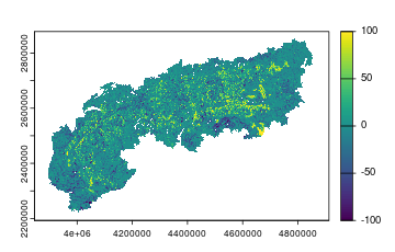
plot of chunk unnamed-chunk-40
Accessibility
This function downloads, processes, and extracts variables from the Global Accessibility Indicators dataset (Nelson et al. 2019). Each variable corresponds to a global raster representing the travelling time (in minutes) to cities or ports of specific sizes.
Available variables (17 total)
Cities:
- 1 - cities1 - cities 1, city 1, cities >5m, huge cities, travel time cities 1
- 2 - cities2 - cities 2, city 2, cities >1m, large cities, travel time cities 2
- 3 - cities3 - cities 3, city 3, medium cities, travel time cities 3
- 4 - cities4 - cities 4, city 4, small cities, travel time cities 4
- 5 - cities5 - cities 5, city 5, travel time cities 5
- 6 - cities6 - cities 6, city 6, travel time cities 6
- 7 - cities7 - cities 7, city 7, travel time cities 7
- 8 - cities8 - cities 8, city 8, towns, travel time cities 8
- 9 - cities9 - cities 9, city 9, small towns, travel time cities 9
- 10 - cities10 - cities 10, city 10, aggregated cities 1, travel time cities 10
- 11 - cities11 - cities 11, city 11, aggregated cities 2, travel time cities 11
- 12 - cities12 - cities 12, city 12, aggregated cities 3, travel time cities 12
Ports:
- 13 - ports1 - ports 1, port 1, large ports, travel time ports 1
- 14 - ports2 - ports 2, port 2, medium ports, travel time ports 2
- 15 - ports3 - ports 3, port 3, small ports, travel time ports 3
- 16 - ports4 - ports 4, port 4, very small ports, travel time ports 4
- 17 - ports5 - ports 5, port 5, any port, all ports, travel time ports 5
processed <- par_set(shape = Alps, crs = 3035) %>%
  accessibility(vars = c("large cities", "ports1"))
plot(processed[[1]])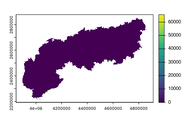
plot of chunk unnamed-chunk-42
GDP past
This function downloads, processes, and extracts variables from the global 1km gridded revised real gross domestic product and electricity consumption dataset (1992–2019) (Chen et al. 2022a).
Available variables (2 total)
Economic metrics:
- 1 - gdp - gross domestic product, real gdp, economy, economic output, gross product
Energy metrics:
- 2 - electricity - electricity consumption, energy, energy consumption, power, ec, electric
Years available: 1992 to 2019.
plot(processed)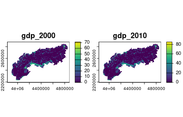
plot of chunk unnamed-chunk-44
Population
This function downloads, processes, and extracts variables from the Global Population Projections dataset (Wang et al. 2022). It provides 1-km grid population distributions from 2020 to 2100 under five Shared Socioeconomic Pathways (SSPs).
Available variables (1 total)
Population Counts:
- 1 - population - pop, inhabitants, residents, people, count, census
Use the arguments year and ssp to filter
the specific data required.
Years available: 2020 to 2100 in 5-year intervals (e.g., 2020, 2025, 2030…, 2100).
SSP Scenarios:
- SSP1
- SSP2
- SSP3
- SSP4
- SSP5
processed <- par_set(shape = Alps, crs = 3035) %>%
  population(vars = "population", year = 2050, ssp = 2)
plot(processed)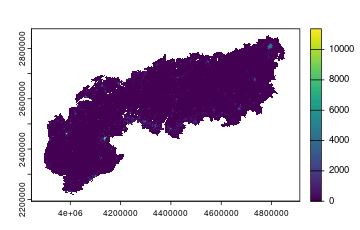
plot of chunk unnamed-chunk-48
Roads
This function downloads, processes, and extracts road density variables from a global dataset of road density at 1 km grid resolution, derived from the OpenStreetMap database (https://www.openstreetmap.org/) accessed through the GeoFabrik (https://www.geofabrik.de/) functionalities. The roads were downloaded from OpenStreetMap as of 30 January 2026. Every layer reports the length in metres of roads within each cell, i.e. road density per 1 km grid cell, and the extent of the data is [-180, 180, -60, 84].
Out of the original OpenStreetMap categories, roads were classified
into five classes, which were then grouped into three further aggregated
layers. Any of these eight layers can be requested through the
vars argument.
Available variables (8 total)
Single road classes:
- 1 - class1 - class 1, roads 1, road class 1, highways, highway, motorway (sum of the original OpenStreetMap categories “motorway” and “motorway_link”)
- 2 - class2 - class 2, roads 2, road class 2, primary class, trunk (sum of “primary”, “primary_link”, “trunk” and “trunk_link”)
- 3 - class3 - class 3, roads 3, road class 3, secondary roads, secondary (sum of “secondary” and “secondary_link”)
- 4 - class4 - class 4, roads 4, road class 4, tertiary roads, tertiary (sum of “tertiary” and “tertiary_link”)
- 5 - class5 - class 5, roads 5, road class 5, quaternary, local roads, local, residential (sum of “residential”, “living_street”, “unknown” and “unclassified”)
Aggregated groups of classes:
- 6 - primary - primary roads, primary group, classes 4 and 5 (sum of classes 4 and 5)
- 7 - other - other roads, other group, classes 1 2 and 3 (sum of classes 1, 2 and 3)
- 8 - all - all roads, total, total roads, all classes, combined (sum of all five classes)
Two details are worth keeping in mind when choosing among these
layers. First, the aggregated layer primary groups the
minor-road classes 4 and 5, and is therefore not the same thing
as the single class class2 (the OpenStreetMap “primary”
category); conversely, the aggregated layer other
groups the major-road classes 1, 2 and 3. This is the naming
used by the authors of the dataset, so vars = "primary"
returns the group and vars = "primary class" (or
"class2") returns the single class. Second, in the three
aggregated layers the cells with no road cover are already stored as NA
rather than as 0, which keeps the files small and speeds up download and
analyses; the five single-class layers instead keep their original
values. As a consequence, all is exactly the sum of
primary and other, and a cell that is NA in
all simply carries no mapped road at all.
If vars is not specified, only all is
downloaded. The layers are hosted in an embargoed Figshare repository
and are retrieved through private links: access is provided for the use
of this package while the repository is under embargo, so please check
with the data authors before redistributing them.
In the example below we download the total road density over Switzerland, projected to EPSG:3035. The Alpine valleys and the densely settled Swiss Plateau stand out clearly.
plot(processed)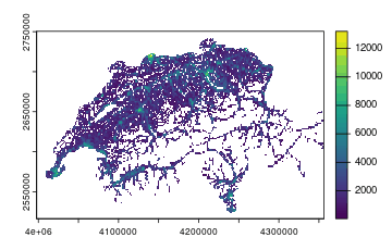
plot of chunk roads-plot
Single classes and groups can also be combined in a single call, and each layer is returned with the name that was requested:
Protected areas
IUCN protected areas
This function downloads, processes, and extracts variables from the World Database of Protected Areas (WDPA) (Planet 2025). Each variable corresponds to a global raster representing different IUCN Management Categories of protected areas.
Available variables (8 total)
- 1 - WDPA_IA - strict nature reserve, strict reserve, 1a, ia, Ia (IUCN Category Ia)
- 2 - WDPA_IB - wilderness area, wilderness, 1b, ib, Ib (IUCN Category Ib)
- 3 - WDPA_II - national park, park, 2, ii, II (IUCN Category II)
- 4 - WDPA_III - natural monument, monument, 3, iii, III (IUCN Category III)
- 5 - WDPA_IV - habitat species management, habitat management, 4, iv, IV (IUCN Category IV)
- 6 - WDPA_V - protected landscape, protected seascape, landscape, 5, v, V (IUCN Category V)
- 7 - WDPA_VI - sustainable use, natural resources, 6, vi, VI (IUCN Category VI)
- 8 - WDPA_ALL - all, combined, full, total, all protected areas (Combined/Full WDPA)
processed <- par_set(shape = Alps, crs = 3035) %>%
  protection(vars = c("national park", "WDPA_ALL"))
plot(processed)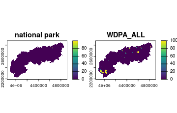
plot of chunk unnamed-chunk-50
Conclusion
This tutorial provided an overview of all the available sources and functions. Remember to always cite the proper reference for the source used. For further details on the use of specific sources, check the function documentation here or from R after loading the package with ? (e.g., ?spectre).
Appendix: A runnable mini-example
Each source above is downloaded on demand, which needs network
access, so those chunks are shown but not executed when
the article is built through GitHub pages at each deploy. However,
whatever the source, every variable comes back as a named layer in a
SpatRaster. To show what that looks like offline, here we
show a real WorldClim (Fick
& Hijmans 2017) extract for Switzerland holding four such
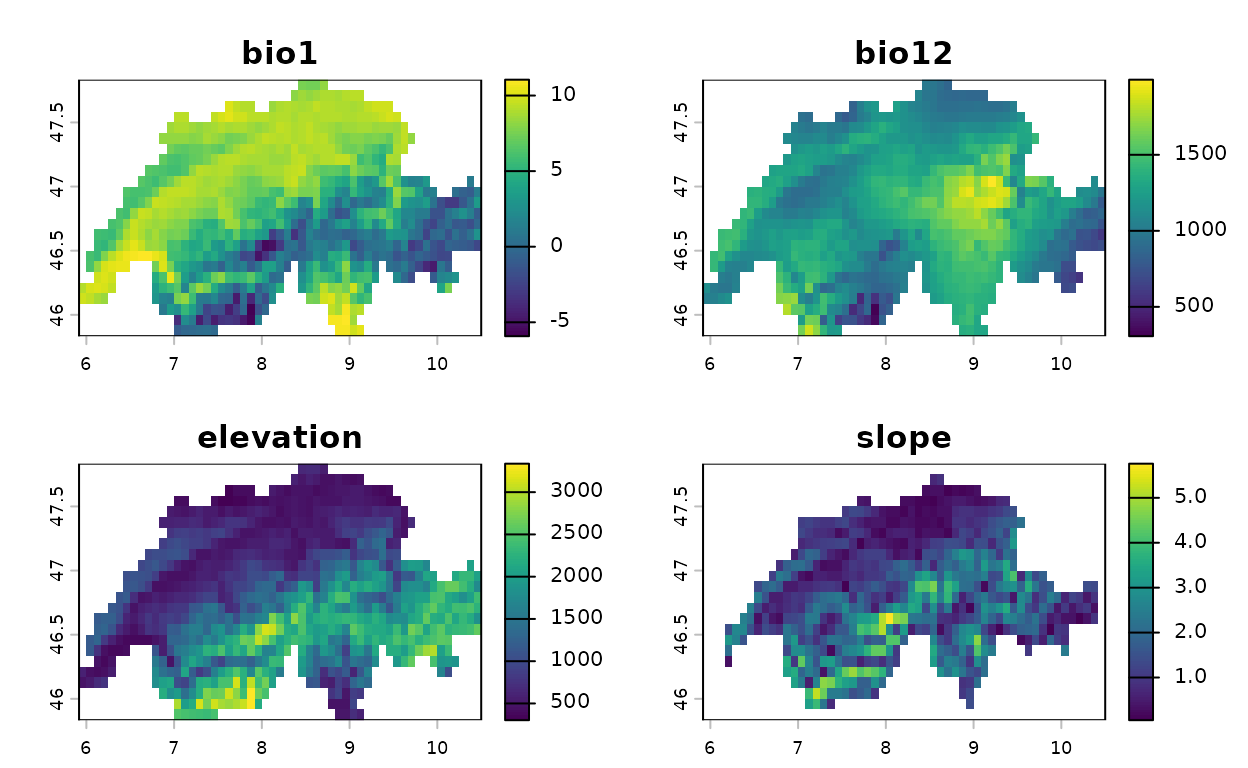
variables — mean annual temperature (bio1), annual
precipitation (bio12), elevation and
slope at ~9 km. The chunk below loads it in place
of a download and inspects the variables it contains.
library(envar)

# A downloaded stack behaves exactly like this bundled one:
switzerland <- terra::rast(
  system.file("extdata", "switzerland.tif", package = "envar")
)

# The layer names are the variable names you requested via `vars = c(...)`:
names(switzerland)
## [1] "bio1" "bio12" "elevation" "slope"
# Per-variable summary statistics over the study area:
terra::global(switzerland, c("min", "mean", "max"), na.rm = TRUE)
## min mean max
## bio1 -5.92 5.224702 11.05
## bio12 307.00 1235.081608 1994.00
## elevation 302.00 1304.183922 3337.00
## slope 0.05 1.612203 5.76
# Plot every variable layer:
terra::plot(switzerland)