Package aims
When conducting an ecological analysis, the response of one or more variable(s) is modeled as a function of one or more predictor(s). When variables are not directly collected in the field or through remote sensing, and information on the spatial location of samples is available, global and already published maps can be used to define variable values. This process is often time-consuming and requires the standardization of different sources to the same study area and/or the extraction of value across study points and/or the conversion to a common coordinate reference system. envar is an R package that allows the download of a wide range of environmental variables from different pre-existing sources, to make the whole process of retrieving variables easier and faster, and integrated within the R environment. The user can thus avoid to manually download and process different variables from different sources, and instead focus on the analysis itself and integrate the downloaded and processed variables within a single R pipeline.
First use: installation
First, we install the package with the following code.
# install using the "remotes" package
if (!require(remotes)) install.packages("remotes")
remotes::install_github("animalbiodiversitylab/envar",
                        upgrade="never",
                        dependencies=TRUE,
                        build_vignettes=FALSE)

# or alternatively using the "devtools" package
if (!require(devtools)) install.packages("devtools")
devtools::install_github("animalbiodiversitylab/envar",
                        upgrade="never",
                        dependencies=TRUE,
                        build_vignettes=FALSE)
Load the library
When executing this command, another package (dplyr)
will be automatically loaded to ensure the full functionality of the
package. However, other packages are often required for plotting and
further analyses and we also load them here for later use.
Full working example
Here, we show a full working example of how to use the package to
download and process a set of environmental variables for a specific
study area. We will download a set of climatic, topographic, and land
cover variables for a study area in the European Alps (already included
in the package as the object Alps()). A call to the
par_set() function is used to define the study area
(argument “shape”), the desired grid output resolution in km (argument
“res”), the coordinate reference system (argument “crs”), and an
eventual buffer (in km) by which to expand the study area (argument
“buffer”). The default resolution is always 30 arcseconds (0.008333333°,
or ~ 1 km) at the equator, except for the biooracle()
function, and “res” specifies a factor by which to aggregate (the
default is 1 and doesn’t apply any change).
Then, the “%>%” is used to concatenate different commands. The next step is to set the specific functions that are used to download and process variables from different sources (see the reference for a full list). The call to a generic source is structured as: sourcename(vars = c()), where sourcename is the name of the function devoted to one source and inside the “vars” argument the specific variables to be downloaded from that source are specified. In this example, we first download a set of 5 bioclimatic variables from the CHELSA source (Karger et al. 2017), then we download elevation and slope from the topography source (Amatulli et al. 2018), and finally we download the percentage cover of trees and ice from the 1 km resolution global land cover based on the ESA 30 m land cover (Lo Parrino et al. 2025).
A correlation analysis can be performed with the to
corr_check() function to identify and remove highly
correlated variables. This function must always be called as the last
one in the pipeline.
It is also possible to call the extr_check() function at
the bottom of the code to enable an automatic test of extrapolation,
regardless of whether you requested already a corr_check().
Ecological models often produce spurious predictions when predicting in
environmental conditions not present in the calibration range (Elith et al. 2010). This problem can
arise under two conditions: 1) at least a variable has values outside
the calibration range - strict extrapolation -, or 2) all variables fall
in the calibration range, but novel combinations of predictor values are
met - combinatorial extrapolation - (Zurell
et al. 2012). Inside the function it is possible to
specify if strict and/or combinatorial extrapolation has to be checked
(argument “type” - default to strict only), and it is necessary to
specify the calibration points as data.frame with X and Y columns
(argument “calib_points”) and the CRS of those coordinates (argument
“calib_crs”) if different from the default (EPSG:4326). Extrapolation is
checked creating an environmental overlap mask, using a method adapted
from Zurell et al. (2012) (Zurell et al.
2012) and implemented natively within envar. To
check extrapolation we assume that a dataset of 2648 occurrences of the
Parnassius apollo butterfly (dataset Apollo()
already included in the package) was used to train any model and that we
want to apply the model to the European Alps later on.
processed <- par_set(shape = Alps, crs = 3035, res = 2, buffer = 10) %>%
             chelsa(vars = c("bio1", "bio4", "bio10", "bio12", "bio19"),
                    years = "1981-2010") %>%
             topography(vars = c("elevation", "slope")) %>%
             melc(vars = c("trees", "ice")) %>%
             corr_check() %>%
             extr_check(calib_points = Apollo, type = "strict")
Output overview
If the correlation and/or extrapolation analysis/es is/are performed, the output is a list. Otherwise, it is a SpatRaster (object to be used within the terra R package), either with a single layer or with multiple layers if multiple variables were specified. If the output is a list, it contains the following elements: “data” (the SpatRaster or data.frame with your data), “correlation_matrix” containing a matrix of Pairwise Pearson’s correlation coefficients between all variables, “vif” a data.frame containing the Variance Inflation Factors for each variable, a “summary” that reports if and which variables have a Pearson’s correlation coefficient higher than |0.6| and/or a VIF higher than 3. The “plot_path” specifies the local directory to which a plot of the Pearson’s pairwise correlation was saved. An “extrapolation” object will then be one layer - two if both strict and extrapolation are checked - reporting as 1 cells of extrapolation and 0 cells of no extrapolation.
# Plot the first two variables
terra::plot(processed$data[[1:2]])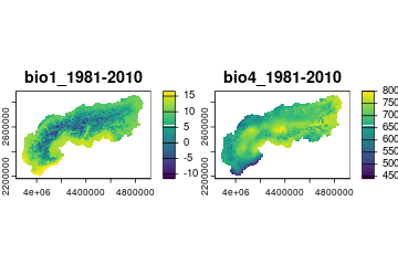
plot of chunk unnamed-chunk-6
# View the Pearson's pairwise correlation matrix
print(processed$correlation_matrix)
## bio1_1981-2010 bio4_1981-2010 bio10_1981-2010 bio12_1981-2010
## bio1_1981-2010 1.0000000 -0.17098433 0.99411075 -0.58856258
## bio4_1981-2010 -0.1709843 1.00000000 -0.06629979 -0.13822734
## bio10_1981-2010 0.9941107 -0.06629979 1.00000000 -0.61255277
## bio12_1981-2010 -0.5885626 -0.13822734 -0.61255277 1.00000000
## bio19_1981-2010 -0.4182732 -0.33185424 -0.45693075 0.84502782
## elevation -0.9682340 0.06664318 -0.96993166 0.58178549
## slope -0.7884759 0.01527641 -0.79705030 0.57544349
## trees 0.1420440 -0.28430061 0.10591260 0.02372563
## ice -0.4765922 0.13185174 -0.46273645 0.27137511
## bio19_1981-2010 elevation slope trees ice
## bio1_1981-2010 -0.418273159 -0.96823403 -0.78847587 0.142043991 -0.4765922
## bio4_1981-2010 -0.331854239 0.06664318 0.01527641 -0.284300607 0.1318517
## bio10_1981-2010 -0.456930752 -0.96993166 -0.79705030 0.105912597 -0.4627365
## bio12_1981-2010 0.845027822 0.58178549 0.57544349 0.023725631 0.2713751
## bio19_1981-2010 1.000000000 0.44083530 0.39996749 -0.003624083 0.2299007
## elevation 0.440835298 1.00000000 0.83277881 -0.120815882 0.4857175
## slope 0.399967493 0.83277881 1.00000000 0.223848319 0.2433729
## trees -0.003624083 -0.12081588 0.22384832 1.000000000 -0.3266344
## ice 0.229900683 0.48571755 0.24337291 -0.326634442 1.0000000
# View the Variance Inflation Factor values
print(processed$vif)
## Variables VIF
## 1 bio1_1981-2010 3073.957200
## 3 bio10_1981-2010 2670.551839
## 6 elevation 40.083967
## 2 bio4_1981-2010 35.854595
## 7 slope 5.865724
## 4 bio12_1981-2010 5.292550
## 5 bio19_1981-2010 4.770264
## 8 trees 1.875957
## 9 ice 1.566896To better understand the structure of correlation, we can also analyze the correlation plot that was locally stored.
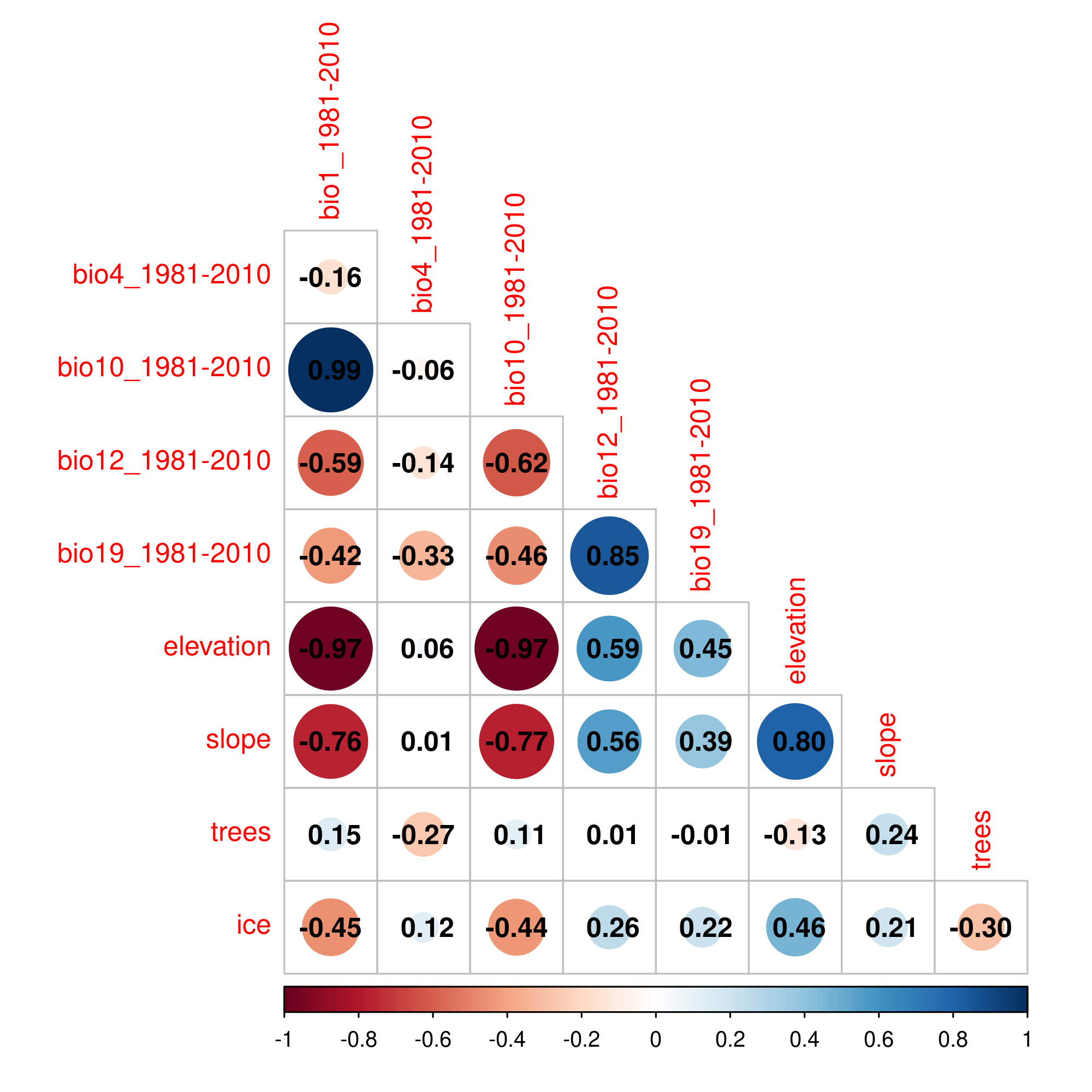
plot of chunk unnamed-chunk-9
This plot was created with the aid of the corrplot R package and it helps to pinpoint correlation problems. In this example, we can see that elevation is highly correlated with multiple variables and as this is not a proximal variable (i.e., the effect of elevation on species distributions is mediated by other co-varying factors such as climate) we can remove it. To obtain a set of uncorrelated variables we might thus want to sub-set our variables as follows.
# define a set of uncorrelated variables
uncorrelated_vars <- processed$data[[c("bio1_1981-2010", "bio12_1981-2010", "trees", "ice")]]
We can also see where extrapolation occurs in our study area. This map can be used alongside any ecological prediction (e.g., species distribution models applied over the European Alps), to interpret more carefully predictions in areas where extrapolation is found.
# visualize the raster map of where extrapolation occurs (1 = extrapolation, 0 = no extrapolation)
terra::plot(processed$extrapolation$strict)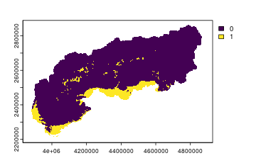
plot of chunk unnamed-chunk-11
Conclusion
We have shown a single full example of use of the envar R package. Instead of specifying a shape, we could have chosen a country/continent or defined a data.frame of points. For an overview of all the possible use-cases see the package overview vignette and for a full list of all the available sources and variables see the reference.
Appendix: A runnable mini-example
Downloading global environmental layers needs network access, so the
download chunks in this article are shown but not
executed when the article is built through GitHub pages. To
keep the package fully reproducible and automatically tested, here you
can also find a test that does not include any download: a WorldClim
(Fick & Hijmans 2017) extract for
Switzerland with mean annual temperature (bio1), annual
precipitation (bio12), elevation and
slope at ~9 km resolution. The chunk below loads it
in place of a download and runs the heart of the
workflow — the collinearity and extrapolation checks — end to end. It is
a miniature of what shown above.
library(envar)

# In a real analysis these layers would come from a download pipeline such as
#   par_set(country = "Switzerland") %>%
#     worldclim(vars = c("bio1", "bio12")) %>% topography(vars = "elevation")
# Here we simply load the equivalent layers bundled with the package:
example_file <- system.file("extdata", "switzerland.tif", package = "envar")
switzerland  <- terra::rast(example_file)
switzerland
## class : SpatRaster
## size : 24, 55, 4 (nrow, ncol, nlyr)
## resolution : 0.08333333, 0.08333333 (x, y)
## extent : 5.916667, 10.5, 45.83333, 47.83333 (xmin, xmax, ymin, ymax)
## coord. ref. : lon/lat WGS 84 (EPSG:4326)
## source : switzerland.tif
## names : bio1, bio12, elevation, slope
## min values : -5.92, 307, 302, 0.05
## max values : 11.05, 1994, 3337, 5.76
# Check collinearity among the layers (bio1 and elevation are strongly related):
checked <- corr_check(switzerland)
checked$summary
## [1] "High Cor (>0.7): bio1, elevation" "High VIF (>3): elevation, bio1"
# Flag environmental extrapolation relative to the Apollo butterfly
# occurrences that fall within Switzerland (used here as calibration points):
calib   <- subset(Apollo, X >= 5.9 & X <= 10.5 & Y >= 45.8 & Y <= 47.8)
checked <- extr_check(checked, calib_points = calib, type = "strict")

# Map mean annual temperature next to where extrapolation occurs
# (1 = novel conditions, 0 = analog conditions):
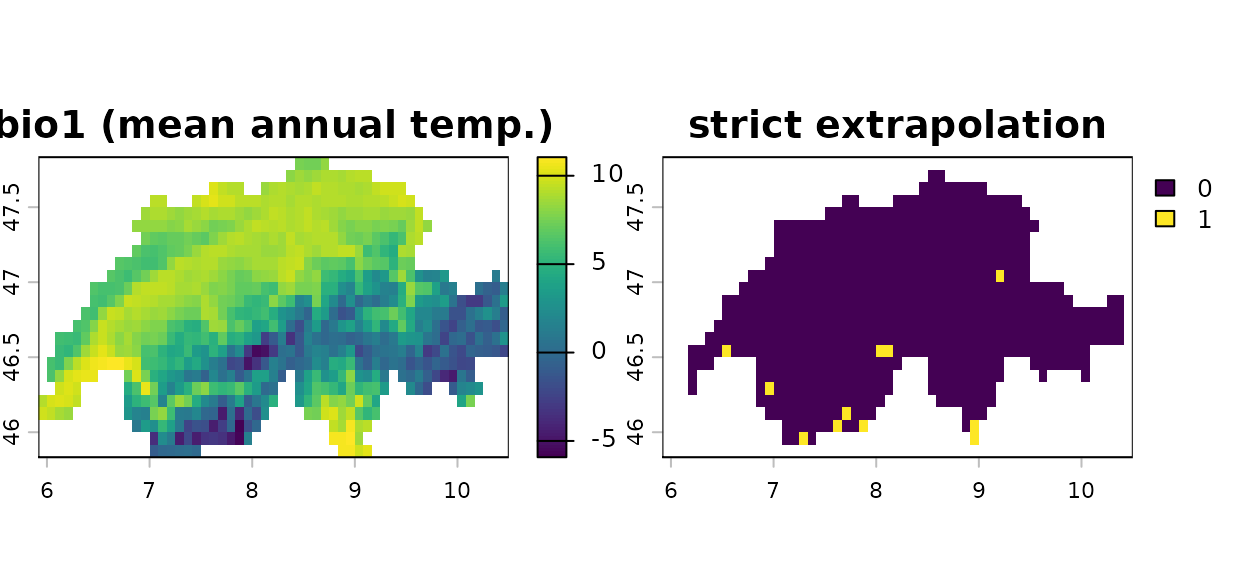
terra::plot(c(switzerland[["bio1"]], checked$extrapolation),
            main = c("bio1 (mean annual temp.)", "strict extrapolation"))